Benchmarking Workload Storage Performance – An Expert Q&A

Nearly 1,000 people have watched our most recent SNIA ESF webcast, Storage Performance Benchmarking: Workloads. We hope you didn’t miss this 5th and final installment of the now famous Storage Performance Benchmarking webcast series where our experts, Mark Rogov and Chris Coniff, explained how to measure and optimize storage performance of workloads. If you haven’t seen it, it’s available on-demand. The live audience had many great questions. Here are answers to them all.

Q. Is it good to assume that sequential IO would benefit from large IO size and, conversely, random IO from small IO size?

A. I don’t think “benefit” is a practical way to look at this. Workloads come in all sizes and mixes, and it is the job of the storage array to handle what is thrown at it. Storage admins (and placement algorithms) need to configure the system to produce the best performance given the current load. Historically, random workloads are harder to optimize than sequential. Mixing block sizes, even with sequential workloads, is also tough to deal with. It all comes to figuring out where the bottlenecks are, and how to overcome them.

Q. But pre-fetch, cache, etc. will show benefit to sequential IO on all Flash array versus random?

A. Technically, we need to look at the effects of cache and pre-fetch on Reads and Writes separately. For Reads, pre-fetching data into cache does show a lot of benefit, especially for sequential IO. For Writes, pre-fetching is not effective, but cache is: it is, generally, faster to save data to cache than straight to disk (assuming, of course, there is free space in cache to write to).

Q. Don’t you see [concatenation of small IOs into larger IO] when apps are inside a VM versus physical nodes? I ask because [block size] changes with versions of hypervisors.

A. This is a great question, and a big misconception floating out there. Hypervisors have three primary methods for accessing storage: direct block, NAS, or via internal filesystem.

The direct block, aka raw device mapping, is simple—all IOs are simply sent to the storage array as they are. No concatenation, folding, compression, etc.

Internal filesystem, VMFS, has a concept of a block size. These blocks are used for internal management of the filesystem (see our File webcast with explanation on how those work). A common misconception is that when a block size is smaller than the write IO size, the filesystem issues a write equal to its block size. In reality, the writes are simply passed to the underlying driver, plus some additional meta-data IO. The amount of data being written doesn’t change just because it is written into a larger block container. In cases when the write IO is larger than a block size of the FS, yes, the storage will see a multiple of IOs, depending on what the ratio is. In VMFS though, block sizes are usually quite large: 1MiB, 4MiB, 8MiB. Very few (if any!) workloads have IOs that big. VMFS also has a concept of “sub blocks”, which are smaller than 1MiB, but are also quite large: 64KiB, with the same logic applied.

NAS communication is the most complex. For the purposes of this question, consider the Ethernet Maximum Transfer Unit size (MTU). It regulates the size of the frame, which by default is 1500 bytes. Therefore, all data must be either smaller than or cut into 1500 byte chunks to be sent across the wire. For example, 4KiB IO will be split into 3 frames: 1500, 1500, and 1096. Sometimes, MTU is set to a “jumbo setting”, or 9000. Then each 4KiB IO will fit into one frame. With NFSv4, the protocol allows combining several NFS calls into one frame. Theoretically, that means that two NFS write calls for 4KiB could fit into a single 9KB jumbo Ethernet frame. In reality, one needs to examine closely which specific NFS calls are truly being used—see our File webcast on details of how block commands get translated to and from filesystem calls and extrapolate that into NFS calls (FS and NFS are not the same!).

Bottom line, regardless of the datastore access method, in most cases, your workload IO will be passed to the storage array as is without coalescing.

Q. There are several other factors that have to be considered: 1) More than random/sequential it’s I/O adjacency that matters most. Think how differently a hybrid storage system would handle random I/O to 5% of the volume vs. even sequential to the whole volume. 2) Does the data dedupe/compress using the array’s algorithm?

A. I agree somewhat with this comment. Adjacency of the IO is a good way to think about things. Intelligent placement algorithms do have a concept of a “Working Area,” which could elect promoting whole regions to the faster storage tier to speed up all the “adjacent” random requests. Data reduction (compression, deduplication, single-instancing, zero-padding, etc.) introduces an overhead in some arrays, and therefore is mudding the picture somewhat, yet the underlying principles remain the same. Keep in mind, this is a vendor neutral presentation, very commonly the differences in handling data reduction are heavily marketed between different solutions.

Q. I think Mark is at a different company now 🙂 2 4 8 is NOT sequential, it is strided, or Geometric. Holistically, If proc A reads 2,4,6 and Proc B read 1,3,5,7 then the strides are within a proc, but holistically, this would be sequential. Though few operating systems do this level of pre-fetch logic.

A. Good catch, and I agree. In a later revision of the slides, we changed the 2, 4, 6 sequence into “predictable” pattern, not sequential.

Q. If you have an all Flash array what kind of performance hit do u take between sequential / random reads? I would think that it isn’t as impactful as a mechanical drive.

A. The answer can be true under one condition and not another (LUN is in a write-pending condition, cache flushing is taking place, etc.).  

Generally speaking, reads always perform better than writes on flash drives.   As for random vs sequential IO, they are measured with two different metrics (iops vs throughput). In order to answer that part of the question, their measurements must be normalized to a common KPI, such that they could be compared.   And to do that, we’d have to know what IO block size the question assumes, as it must be known to solve for ‘IO size x IOPS = Throughput in MB/s’

This is from the spec sheet for one vendor’s SSD:

  • Sequential Read (up to)450 MB/s
  • Sequential Write (up to)380 MB/s
  • Random Read (100% Span)67500 IOPS
  • Random Write (100% Span)17500 IOPS
  • Latency – Read40 µs
  • Latency – Write42 µs

So, the ‘It Depends” answer is based on the manufacture & model of drive at specific code level, and (if it’s in an array) how the specific array vendor implemented it in their design.   If it’s an Integrated Cache Disk Array (ICDA), then pre-fetching (read ahead) and caching algorithms behave differently at various code levels for each vendor.  There are specific used defined configuration parameters that can negate the answer to the question below as well.   For instance, High & Low water marks, Dynamic Cache Partitioning, Workload QoS, etc.

In the case of an ICDA, what’s more important than read vs write or random vs sequential is whether or not the IO was a cache hit.  A cache hit for a single random read IO in an ICDA who’s LUN is on a 7.2K SATA drive will have better performance than a random read miss on that same array if the LUN were on a flash drive.

So, as we’ve seen throughout this series, there is more to the overall performance benchmark than any one variable.

Q. What observations do you have on rebuild time for Flash disk? On what magnitude is it faster than spinning disks considering a high-end hybrid or AFA storage system?

A. This question is dangerous, as it crosses into vendor specifics. Rebuild time depends on more than just the type of drive, the RAID type and configuration, drive utilization, array business—and many more factors come into play here. Generally, an SSD drive will rebuild faster than a similarly sized spinning drive.

Q. What about the fact that you get cache effects in the OS stack and also in the Flash (DRAM landing areas) that actually improves write latency versus reads? Isn’t it worth mentioning Writes can actually appear higher performant on Flash? Or am I missing something? (Probably the latter) 🙂

A. You are 100% correct! 🙂 But do consider the size of DRAM… how much data can it take? Does the entire “working area” fit there? If it does, viola! If it does not – welcome to the rest of the world!

Q. Can you send links to all the webcasts in this series?

A. Of course, please see below and happy viewing!

  1. Storage Performance Benchmarking: Introduction and Fundamentals
  2. Storage Performance Benchmarking: Part 2  – Solution under Test
  3. Storage Performance Benchmarking: Block Components  
  4. Storage Performance Benchmarking: File Components  
  5. Storage Performance Benchmarking: Workloads

Storage Performance Benchmarking: Workloads

The SNIA Ethernet Storage Forum is very pleased to announce that the hugely popular “Storage Performance Benchmarking” webcast series continues with a 5th installment! Join us on February 14th at 10:00 am PT for “Storage Performance Benchmarking: Workloads.”

Benchmarking storage performance is both an art and a science. In this 5th installment, our experts, Mark Rogov and Chris Conniff, take on optimizing performance for various workloads. Attendees will gain an understanding of workload profiles and their characteristics for common Independent Software Vendor (ISV) applications and learn how to identify application workloads based on I/O profiles to better understand the implications on storage architectures and design patterns. This webcast will cover:

  • An introduction to benchmarking storage performance of workloads
  • Workload characteristics
  • Common Workloads (OLTP, OLAP, VMware, etc.)
  • Graph fun!

Did you notice this webcast is on February 14th? We did that on purpose, because we know you’ll love it! So, register now and spend an hour of your Valentine’s Day with us. We hope to see you there.

And if you have not yet had a chance to watch any of our previous “Storage Performance Benchmarking” webcasts, they are all available on-demand.


An FAQ to Make Your Storage System Hum

In our most recent “Everything You Wanted To Know About Storage But Were Too Proud To Ask” webcast series – Part Sepia – Getting from Here to There, we discussed terms and concepts that have a profound impact on storage design and performance. If you missed the live event, I encourage you to check it our on-demand. We had many great questions on encapsulation, tunneling, IOPS, latency, jitter and quality of service (QoS). As promised, our experts have gotten together to answer them all.

Q. Is there a way to measure jitter?

A. Jitter can be measured directly as a statistical function of the latency, typically as the Variance or Standard Deviation of the latency. For example a storage device might show an average latency of 5ms with a standard deviation of 1.5ms. This means roughly 95% of the transactions have a latency between 2ms and 8ms (average latency plus/minus two standard deviations), however many storage customers measure jitter indirectly by showing the 99.9%, 99.99%, or 99.999% latency. For example if my storage system has 99.99% latency of 8ms, it means 99.99% of transactions have latency <=8ms and 1/10,000 of transactions have latency >8ms. Percentile latency is an indirect measure of jitter but often easier to calculate or understand than the actual jitter.

Q. Can jitter be easily characterized for storage, media, and networks.   How and what tools are available for doing this?

A. Jitter is usually easy to measure on a network using standard network monitoring and reporting tools. It may or may not be easy to measure on storage systems or storage media, depending on the tools available (either built-in to the storage OS or using an external management or monitoring tool).   If you can record the latency of each transaction or packet, then it’s easy to calculate and show the jitter using standard statistical measures such as Variance or Standard Deviation of the latency. What most customers do is just measure the 99.9%, 99.99%, or 99.999% latency. This is an indirect measure of jitter but is often much easier to report and understand than the actual jitter.

Q.  Generally IOPS numbers are published for a particular block size like 8k write/read size, but in reality, IO request per second could be of mixed sizes, what is your perspective on this?

A. Most IOPS benchmarks test only one I/O size at a time. Most individual real workloads (for example databases) also use only one I/O size.  It is true that a storage controller or HDD/SSD might need to support multiple workloads simultaneously, each with a different I/O size.  While it is possible to run benchmarks with a mix of different I/O sizes, it’s rarely done because then there are too many workload combinations to test and publish. Some storage devices do not perform well if they must handle both small random and large sequential workloads simultaneously, so a smart storage controller might assign different workload types to different disk groups.

Q. One often misconfigured parameter is queue depth. Can you talk about how this relates to IOPS, latency and jitter?

A. Queue depth indicates how many tasks or I/Os can be lined up for a particular resource, such as a storage controller, network interface, or CPU. Having a higher queue depth ensures the resource stays highly utilized because it always has a new task to do as soon as it finishes its current task(s). This can result in higher IOPS because the CPU is less likely to have idle time waiting for new tasks to be put into its queue. But it could also increase latency because longer queues mean each task spends more time waiting in a queue.  It’s easy to misconfigure queue depth because you it needs to be deep enough to keep the resource (CPU/controller/interface) busy but not so deep that each transaction spends a long time in the queue.

Q. Can you please repeat all your examples of tunneling? GRE, MPLS, what others? How can it be IPv4 via IPv6?

A. VXLAN, LISP, GRE, MPLS, IPSEC.   Any time you encapsulate and send one protocol over another and decapsulate at the other end to send the original frame that process is tunneling. In the case we showed of IPv6 over IPv4, you are taking an original IPv6 frame with its IPv6 header of source address to destination address all IPv6 and sending it over and IPv4 enabled network we are encapsulating the IPv6 frame with an IPv4 header and “tunneling” IPv6 over the IPv4 network.

Q. I think it’d be possible to configure QoS to a point that exceeds the system capacity. Are there any safeguards on avoiding this scenario?

A. Some types of QoS allow over-provisioning and others do not. For example a QoS that imposes only maximum limits (and no minimum guarantees) on workloads might not prevent many workloads from exceeding system capacity. If the QoS allows over-provisioning, then you should use system monitoring and alerts to warn you when system capacity has been exceeded, or when any workloads are not getting their minimum guaranteed performance.

Q. Is there any research being done on using storage analytics along with artificial intelligence (AI) to assist with QoS?  

A. There are a number of storage analytics products, both third party and storage vendor specific that help with QoS. Whether any of these tools may be described as using AI is debatable, since we’re in the early days of using AI to do much in the storage arena. There are many QoS research projects, and no doubt they will eventually make their way into commercially available products if they prove useful.

Q. Are there any methods (measurements) to calculate IOPS/MBps in tier capable storage? Would it be wrong metric if we estimate based on medium level, example tier 2 (between 1 and 3)?

A. This question needs refinement, since tiering is sometimes a cache model rather than a data movement model. And knowing the answer may not actually help! Vendors do have tools (normally internal, since they are quite complex) that can help with the planning of tiered storage.

By now, we hope you’re not “too proud” to ask some of these storage networking questions. We’ve produced four other webcasts in this “Everything You Wanted To Know About Storage,” series to date. They are all available on-demand. And you can register here for our next one on July 6th where we’ll bring in experts to discuss:

  • Storage APIs and POSIX
  • Block, File, and Object storage
  • Byte Addressable and Logical Block Addressing
  • Log Structures and Journaling Systems

The Ethernet Storage Forum team and I hope to see you there!

Update: If you missed the live event, it’s now available  on-demand. You can also  download the webcast slides.


A Q&A on Storage Performance Benchmarking: Block Components

For the third time, our storage performance benchmarking experts, Ken Cantrell and Mark Rogov, have generated an abundance of interest (in the form of questions) on block storage performance. If you missed the Webcast, “Storage Performance Benchmarking: Block Components,” it’s available on demand. It was no small effort to answer all the great questions that we received. And for those of you who have been waiting, we apologize, but we think the detailed and thoughtful answers Mark and Ken have put together are well worth the wait.

Q1: Are these numbers applicable to the 90th percentile for any given storage array, please?

Mark: These numbers represent HDD/SSD performance numbers. They aren’t meant to represent any particular storage array vendor’s performance. See the end of our presentation (bottleneck analysis) as to why it is really really hard to answer your question.

Q2: How about NVDIMM-F or NVDIMM-P or NVDIMM-X claiming 3-4M IOPS type of Enterprise storage devices?

Ken: Yup. They’re fast.

There’s a great presentation by Jim Handy titled “Understanding the Intel/Micron 3D XPoint Memory” presented at SDC2015 that I’d recommend you take a look at to understand more about this kind of memory and its possible positioning.

Mark: Great question. I think the conclusion of our presentation answers it. Flash (and we use flash as a collective term, defining everything that is not spinning storage to be “flash”) is drastically faster than spinning drives. But even within Flash, there are plenty of new technologies which compete with each other and improve the overall performance landscape. So, within the scope of our presentation, even a simple good old SLC drive tops the capability of a SAS line. If we improve on one drive, by switching the technology to a faster/newer/better variant (e.g., NVDIMM-F), or by stacking the drives, the resulting set will much more likely expose the limitations of the “regular” storage array.

Q3: I’d like to know which tool you are using to measure IOPS if possible.  

Ken: The SNIA Solid State Storage Initiative (SSSI) has developed substantial expertise in the area of SSD performance and behavior. The SSS Performance Test Specifications were developed by the SNIA SSS Technical Work Group (TWG) and define how to measure SSD performance in a manner that is accurate, repeatable and enables comparison between different manufacturers’ products. Learn more about the SSD Performance Project here.

All of the Flash and HDD numbers at the beginning of the presentation were taken directly from the Solid State Storage Performance Test Specification summary results (SSS PTS). The SSS PTS provides a comprehensive method for measuring flash performance in the most vendor neutral approach that I’ve seen.

The Flash and HDD numbers at the end of the presentation were 80% of the starting numbers – scaled down to make them slightly more like what we’ve seen in a greater number of environments (that aren’t pushing their drives as hard).

Q4: Throughputs with SSD is not as much as one can get from a spinning drive when one keeps cost/GB on the axis. Comments please.

Ken: Now we have 3 axes? I’m not even sure how to visualize what you’re asking, but I’m pretty sure I understand the intent … and this is a harder question than it would appear on the surface. Why?

  • First off, prices aren’t my thing – I tend to focus on the internals and let the sales guys talk prices. Additionally, vendors often engage in significant discounting or bundling that makes it difficult for the average person (i.e., me) to understand true costs.
  • The astounding random I/O performance of flash enables support for compression and deduplication without dramatically increasing client-perceived latency. There’s a reason you see so many vendors offering inline deduplication and inline compression now when they did not even five years ago – flash is the enabler that makes this happen. So what is the true comparison? Raw HDD vs Raw flash? Or Raw HDD vs flash plus the storage efficiency (SE) savings it enables? If flash with SE features (dedupe and compression), then what is the savings that you can/should expect for your dataset? 1.5x? 5x? 50x? Knowing this is a prerequisite to answering the question, and the answer will be dependent both on the vendor’s features and your own data set characteristics.
  • As we discussed in the first session, if your application/user base have some sort of minimum performance expectations, particularly around latency, then HDDs may simply not be able to provide you the performance you need. You DID mention throughput (IOPS?) explicitly and with IOPS, OPS, or data rates (MB/s), you can always match flash data rates with HDDs – it just might take a LOT more HDD drives than flash devices. Latency/response time is different though – depending on whether you are drive bound and what your I/O characteristics look like (read vs write, random vs sequential), you may simply be unable to ever hit your latency targets with HDD.
  • The world, it is a-changing. six years ago it was easy to say “SSD for performance sensitive niche applications!” and smile. Today, prices continue to drop, vendors are making new decisions around the use of consumer grade vs enterprise grade flash, and overall flash/SSD is moving much more mainstream. And … consider the new 16TB (yes 16 TERABYTE) SSD drives announced by Samsung. My personal view (and I’m explicitly disclaiming that I’m speaking on my behalf, and not NetApp’s – which honestly, you should assume for all my answers) is that these are going to change the landscape almost as dramatically as SSD itself has.
  • There are definitely vendors that believe in the cost benefits of HDD. We chose not to mention specific vendors in the webcast, but consider BackBlaze. In their blog, they are extremely open about how they have configured their data center – and they are an (all?) HDD shop. In fact, “by the end of 2015, the Backblaze datacenter had 56,224 spinning hard drives containing customer data.” Speaking of Backblaze, you might be interested in their assessment of the 16TB drive, for their shop.

You might also be interested in slide 21 of the following, which includes some price/performance numbers from EMC and Oracle.

Q5: Does NVMe drive technology move things to a higher level?

Ken: If you truly mean NAND-based flash accessed via NVMe instead of SAS/SATA, yes. Look at the perf results linked out of question 3. If you mean the use of next-generation non-volatile memory (NVM) instead of NAND-based flash, then yes. The following chart is contained in a lot of SNIA presentations; I It does a good job of pointing out just how much faster we can get.

I also strongly recommend a look through of Advances in Non-Volatile Storage Technologies by Tom Coughlin from Coughlin Associates. If you care about these topics, the SNIA Storage Developer Conference is a great opportunity to learn more.


Performance Benchmarking 3 Graphic

Q6: Why NAND gates and not AND gates?

Mark: NAND and NOR gates are known as “universal gates”–they can be combined in various groups and combinations to do any basic operations, i.e., AND, NOT, OR, etc. So, flash manufacturers had to choose between NAND and NOR. And just like with any technology, the price drove the choice. NAND gates are simply cheaper and slower. NORs are faster and more expensive. Actually, there are some NOR products in the market.

Q7: Mark accidently said 15K was 15,000/sec when it’s 15,000/minute.

Ken: Thanks! (Shame on you Mark!)

Mark: Thank you… I can’t believe that I misspoke! I never do! Never! Ahh!!!

Mark’s Lawyer: On behalf of my client, I move to remove this question and the digital recording from Exhibit A to Exhibit B (aka “never again section”)

Q8: Do you guys have any data about how expensive an erase-modify-write operation is, compared with spinning disks in terms of performance?

Ken: This is what we were attempting to demonstrate in the first set of slides. The PTS (see question 3) forces flash devices into a steady state mode where they are continuously doing program-erase cycles. So the results shown there demonstrate the difference between HDD writes (seek, spin, write) and flash writes (erase and program).

Your question made me wonder though … so I also did a quick literature search. Interesting to see how rates have changed over time, and how they vary by device:

From M-Systems, in 2002: Erase cycle was 3ms

From Micron, in 2006: The erase time for a 128KB erase block was 500 µs

From AnandTech, in 2012: Erase time for SLC was 1.5-2ms, MLC was 3ms and TLC was ~4.5ms (huh? SLC vs MLC vs TLC?)

Q9: Why can’t the pointer be at the page level instead of a block level (say, metadata within a block)? I’m sure that there is a reason. What do we gain by treating an entire block as a monolithic?

Mark: This is an excellent question to ask Google. I think the reasons for selecting a NAND gate technology, and for bundling a bunch of NAND gates into groups and for creating blocks (in essence, super groups) is power. It takes less power to operate the drives with NAND gates and blocks.

Q10: I heard someone mention NOR gates, instead of NAND, are NOR gates persistent, over a power cycle?

Ken. Yes.

Mark: There are plenty of other “Logic gates” see this article on Wikipedia for more information.

Q11: So, there is no advantage in keeping IO sequentially in an SSD?

Ken: Technically, or practically?  Technically speaking, I think it does matter. Micron documented this in 2006, noting that “Random access time on NOR Flash is specified at 0.075μs; on NAND Flash, random access time for the first byte only is significantly slower—25μs (see Table 2 on page 5). However, after initial access has been made, the remaining 2111 bytes are shifted out of NAND at a mere 0.025μs per byte.” The raw numbers have changed over the years, but I don’t believe the principle has.  Violin Memory stated in 2013 that, “The idea of sequential I/O doesn’t exist with flash memory, because there is no physical concept of blocks being adjacent or contiguous. Logically, two blocks may have consecutive block addresses, but this has no bearing on where the actual information is electronically stored. You might therefore say that all flash I/O is random, but in truth the principles of random I/O versus sequential I/O are disk concepts so they don’t really apply.”

Practically speaking, I agree. Sequential vs random I/O is irrelevant for flash. Given (a) average I/O sizes for workloads and (b) the incredible performance of flash devices compared to the needs of the vast majority of people using them, it doesn’t much matter if you can access subsequent bytes in a NAND-based flash device faster than you can access the first bytes. They are plenty fast enough.

Note that it is hard to find public info on this. Sequential I/O tends to use larger I/O sizes, and random I/O uses smaller I/O sizes. So finding apples-to-apples comparisons between sequential and random I/O is difficult.

Mark: Yes, the flash drive doesn’t care anymore. But the hosts and application still do. Where it matters is in the workloads. Ken and I are still planning to dedicate an entire hour talking about workloads, and Random vs. Sequential will surely be a large part of it. However, we will admit that in the future, when all storage will be flash (which is, of course, a pipe dream) it won’t matter anymore.

Q12: What is the acceptance level to Erasure Coding, and hence the change in the way Storage Performance testing will change?

Mark: As we said during the webcast, RAID is a special case of Erasure Coding. Therefore its acceptance rate is 100% J But on a more serious note, Erasure Coding is necessary for any scale out system: and every vendor uses their own N+M rules.

Q13: Is RAID-1 always half the write performance? If the writes go to both drives simultaneously, I could see write performance being less than 100% of what one drive can do, but not half.

Ken: This was asked in a dry run as well. You’ve hit on something that seems to be a sticking point for multiple people.  Perhaps consider it this way. It looks mathy and complicated, but bear with me …

Consider two physical drives. Call them P1 and P2.

Let the write performance (in iops) of P1 be P1w.

Let the write performance (in iops) of P2 be P2w.

How fast can P1 write? P1w.

How fast can P2 write? P2w.

If you can write to both P1 and P2 at the same time, independently, and completely in parallel, how fast can you write in aggregate? P1w + P2w.

For the previous question, what if P1w = P2w?

Then P1w + P2w = P1w + P1w = (2)*P1w.

Now …

Consider a RAID-1 pair comprised of the same P1 and P2. Call it R1.

Writes can be sent (in a good implementation) to both P1 and P2 at the same time.

But, before a write is considered complete, it must be acknowledged by BOTH P1 and P2.

If P1w > P2w, what is the best performance of R1? P2w. P2 is slower, so we’ll always be waiting on it (assuming performance is consistent), so the best we can do is P2w.

Same logic if P1w < P2w.

What if P1w = P2w? What is the best performance of R1? Same logic … but since they are the same speed, it is simply P1w.

So …

In the non-RAID-1 case, our performance (assuming P1w = P2w) was 2 * P1w.

In the RAID-1 case, our performance (assuming P1w = P2w) is P1w.

50% reduction.

RAID-1 only achieves ½ of what the physical pair could.  

Mark: What Ken said.

Q14: Is there any kind of “asynch” RAID1 so that I can keep the performance of the disks but keep the mirroring?

Ken: See the previous answer also.

For reads, certainly. For writes, not that I know of, although you can make it much less visible. For example, if you have a caching RAID controller/system, your writes will go to memory and then go to disk whenever the controller/system decides to flush it. Perhaps it is big enough that it turns random I/O into sequential I/O (and you’re on HDDs) and the perf improvement from doing sequential instead (instead of random) is enough you don’t notice the effect of RAID itself.

Mark: I think that in reality, the behavior of a particular implementation is always vendor-dependent. Generally speaking, RAID1 does allow the reading from both drives, but budgets or software bugs or just plain ignorance could result in an implementation where that is not true. Address vendor documentation to know for sure.

Q15: Why do you need to read old parity to recalculate and write a new one? Isn’t the parity only calculated based on the data being written?

Ken: See answer to question #14.

Mark: It is a math trick… reading the parity saves reading the rest of the blocks on the full stripe. With 3 drives the savings are non-obvious, but with 5 or 14 there are significant.

Q16: This calculation is correct for 3 disks, right? If there are more disks and partial write is for stripe on single drive then you need to read more to calculate parity

Ken: No. There are some great write-ups about how RAID-5 works. Instead of pasting those here, I strongly encourage you to visit http://rickardnobel.se/how-raid5-works/ AND http://rickardnobel.se/raid-5-write-penalty/ and then tweet Mark (@markrogov) or Ken (@kencantrelljr) with questions/follow-up.

(I have no connection to Rickard … I just think he’s done a great job in his write-up.)

Mark: Yes, Rickard’s write up is spot on. Our goal is to introduce a fairly complex subject in a deceivingly simple manner. There are many edge cases that we don’t address: partial write to sector, partial write to a block, partial write a stripe… all those have their own consequences, and storage vendors deal with those differently.

Q17: I am also interested in Data Recovery on NAND technology

Ken: Me too. It isn’t a topic we’re planning to cover though.

Q18: Does caching write data help when one uses SSD?

Ken: It can. Memory is still faster than flash. It depends entirely on how the memory is used. For example, with writes, if memory were used as a write-through cache (look it up if you need), it wouldn’t make things faster. If it were used as a write-back cache, it would. If it is used as a read cache, it will almost certainly make reads of data faster. But even there, life is never simple. Why? Because if you’re using memory to cache data, you’re not using it for something else … and it is possible that the memory could be better used for caching metadata, for example.

Mark: Here, I’d like to recall our good friend, Dr. J Metz, who created an excellent presentation on comparing computer caches to pizza delivery in “Life of a Storage Packet (Walk)” And in his example, caching will keep the pizza warmer. Even if a flash drive is used.

Q19: If the customer is interested in throughput in MB/s then they probably won’t do IOs with 4KB size…

Ken: Agreed. I’m fairly certain that you’re referring to adding MB/s numbers on slide 41. We had a discussion about doing that when putting the slides together. The transition between slide 40 and 42 changed the I/O size from 4KiB to 128KiB, changed from writes to reads, and changed from random I/O to sequential I/O. Adding the MB/s numbers to slide 40/41 was meant to ease the transition between slide 40 and 42. You’re absolutely right though … rarely does anyone want to talk data rates (MB/s) when using small I/O sizes.

Mark: Agreed. Although a true performance guru would recognize that these are the two sides of the same coin.

Update: This webcast is part of a series on storage performance benchmarking. Check out the others:

Storage Performance Benchmarking Q&A – Take 2

Our recent Ethernet Storage Forum Webcast, “Storage Performance Benchmarking: Part 2,” has already been viewed by more than 500 people. If you haven’t seen it yet, it’s now available on –demand. Our expert presenters, Ken Cantrell and Mark Rogov did a great job fielding questions during the live event, but of course there wasn’t time to get to them all. So, as promised here are their answers to all of them. If you have additional questions or thoughts, please comment on this blog and we’ll get back to you as soon as we can.

Q: “As an example, am I right to presume workloads are generated by VMs”

A: Ken: It is probably a good idea at this point to define a workload, since we continue to use the term. At a very high level, think of a workload as the mix of operations issued by an application related to the accessing of data. In our case, data stored or made available by a storage solution. With that in mind, absolutely, workloads can be generated by VMs. But they don’t have to be. In other words, “it depends.”

For example, consider these 3 cases:

1) If your SUT (solution under test) was just a simple laptop with no hypervisor and a traditional OS, then there would be no VM in the mix. Your workload would be generated by the application you were measuring (whether that was a simple file copy or something complex like a local database installation).

2) Your SUT is composed of a physical client (like the laptop above) attached to a machine with a hypervisor installed on it and a local guest OS installation that is capable of exporting NFS or SMB shares. The laptop sends I/O via Ethernet to the guest OS. In this example, there is a VM, but it is acting as the storage system, not the workload generator.

3) Now reverse the I/O of example 2. Have the laptop export an SMB share and have the guest OS issue I/Os to that share. Now you finally have VMs generating workloads.

A: Mark: If one examines the solution under test (SUT), and considers the general data flow, then the workload is generated by the clients/hosts layer. Yes, we indicated that the clients/hosts can be VMs, but they also could be physical systems, and, in the case of a SUT consisting of just one laptop, the workload is generated by the application.

Q: Are you going to get around to file performance benchmarking? This infrastructure stuff is not new to me. I have done block all my life, I am interested in stuff about file.

A: Ken: That’s the plan. We are still working out the exact sequence, timing and content for future presentations, but had a dedicated section on both block and file on the original roadmap. If you have specific topics within “file” that you’d like covered, respond in the comments. No promises to cover them, but knowing the desires of the audience is always a good thing.

Keep in mind the intention of the webcast series – lay a strong, but simple foundation, for storage performance fundamentals and then build on that foundation.

A: Mark: The main intent of the series is to lay down basic performance principles first, then build on them to go to more complex topics. Both Ken and I refer to ourselves as “File Heads” and we can’t wait to concentrate on just file, but it would only make sense given that the infrastructure foundations are firm and understood by our audience.

Q: Why doesn’t SPEC SFS have performance testing for such failure models?

A: Ken: Brighttalk provided this comment in isolation, so it isn’t entirely clear which failure models you’re asking for.  I’m assuming you mean a failure like a drive or controller failure. With that assumption, that said, the SFS subcommittee welcomes publications that illustrate a failure condition. SPEC SFS 2014 provides an excellent opportunity for someone to publish once in a non-failure scenario and then again in a failure condition of some sort – as long as that failure condition doesn’t violate any of the run rules regarding stable storage and the failure condition doesn’t generate user visible errors.

Note that SPEC SFS 2014 doesn’t mandate any demonstration of failure scenarios. We’ve discussed this in the past, but it has never been a priority for those that participate in SPEC (which is open to all – see http://www.spec.org for instructions on how to join the SPEC Open Systems Group).

Q: Why is write cache turned off for enterprise drives?

A: Ken: I knew this question was coming. 🙂 This is related to “stable storage” – the guarantee from your storage provider that data they say is safely stored on disk is actually stored on disk. I should clarify that the comment is a little dated and refers to caches designed around volatile memory; this wouldn’t apply to a hybrid SSD/spinning media drive that used the SSD to cache/stage data, since SSDs are non-volatile.

Consider the failure scenario where the enterprise drive has write caching enabled and then experiences a power failure. In most every system sold, the storage controller treats drives pretty much as black boxes – they tell the drive to read or write data at a certain location and expect the drive to do as told. So, when the drive says “yup, I got that data, you’re good!” the storage solution trusts the drive and, when it doesn’t need it in memory any longer, throws it away (that data is safely stored on disk, so this is ok). If the drive chose to cache that information in volatile memory, and loses power, the information is gone.

Midrange and enterprise storage vendors often (I think I can say generally) provide some sort of battery backup in case of power failures. These battery units keep power to at least some of the drives – but remember that drives (especially spinning ones) suck down a lot of power, and often the implementation chooses to keep power only to certain drives that the storage controller uses to flush its own volatile memory structures to.

A quick Internet search shows some specific comments on this topic:

From Seagate (http://knowledge.seagate.com/articles/en_US/FAQ/187751en):

Windows 2000 Professional / Server, Windows XP Home / Professional, Windows Vista and Windows 7 have a nifty little feature called write caching buried within the depths of property tabs. Normally, this type of feature is used with SCSI drives in server applications to provide greater data integrity.

When drives employ write-back cache, any interruption of power to the drive or system may cause lost or corrupted data because the drive does not have time to write the cached data to the disk before the power is lost. However, when write cache is turned off, drive performance slows down.

From Microsoft (https://support.microsoft.com/en-us/kb/259716):

…In addition, enabling disk write caching may increase operating system performance. This article describes how to enable or disable disk write caching…

NOTE: Enabling write caching generates the following warning. This is normal:

By enabling write caching, file system corruption and/or data loss could occur if the machine experiences a power, device or system failure and cannot be shutdown properly.

Q: What’s the difference between CPU and ASIC? When to use which word?

A: Ken: Unfortunately, the SNIA dictionary doesn’t define either term. At the easiest level, both are acronyms. CPU = central processing unit, and ASIC = application specific integrated circuit. At the next level, think of a CPU as general purpose processing element and an ASIC as a custom designed microchip designed for a special application or purpose. Once created, ASICs are non-programmable – they do something very specific (and hopefully very well and very quickly/efficiently). A CPU can run your bitcoin mining program overnight, wake you to Spotify in the morning, let you use your favorite word processor in between games of Plants vs. Zombies, and still let you watch Hulu before you head off to bed.

An ASIP (Application Specific Instruction-Set Processor) bridges the gap between a general purpose processor (CPU) and the highly specific, targeted design of an ASIC. An ASIP will have a much reduced instruction set and a more targeted design towards a specific application (say, digital signal processing), but still allow the execution of a specific instruction set given to it.

Q: Can you mention tools to identify the bottlenecks?

A: Ken: We are trying very hard, particularly in the webcasts themselves, to stay vendor neutral. I don’t mind violating that though here in the Q&A a little bit.

From an open source standpoint, there are a number of tools. One of the more popular now is to use something like Graphana  as a front-end to Graphite, and use that to monitor a set of open source (or privately designed) sensors, including sensors from OPM below, that you place throughout your environment.

Here are a few other open-source benchmarking and performance tools, and what aspect of performance to which they apply. Please note that this is not a comprehensive list, nor is this a recommendation for their use. We are providing the link as a convenience, not an endorsement. [http://www.opensourcetesting.org/performance.php]

Still free, but NetApp-centric, is OnCommand Performance Manager (OPM), specifically OPM v2.0 and later. In addition to providing performance metrics for your NetApp storage array, OPM offers up the concept of a “bully” and “victim” scenario – it specifically watches for components that are performing poorly (the “victims”) and helps identify which other components are causing that poor behavior (the “bullies”). My team helps develop OPM.

Not free, and not NetApp centric, but a NetApp product, is OnCommand Insight (OCI). This is a premier product for looking at the performance of the components across your datacenter.

A: Mark: I didn’t want to break the vouch to neutrality. 🙂 EMC has a number of tools as well, vRealize suite, ViPR SRM, Unisphere, plus platform specific tools… However, it has been my experience that the most important tool a performance expert has is still the critical mind. One observes the problem, and then walks the entire set of the SUT layers looking for incongruences. Too often, the perceived bottleneck is not the problem, but a manifestation of a problem somewhere else. For example, as we pointed in the “MiB/s section” of this webcast, the network layer was a bottleneck due to the badly configured OS multipath drivers. Deciphering cause from reason requires several things: a good understanding of the SUT and its layers; a critical mind to analyze problem conditions; and a large dose of curiosity. The latter one a personal trait that drives us to question “what if I change this to that?” Asking questions while troubleshooting is, IMHO, a cornerstone requirement and inherently, a very human trait. My personal view is that tools are just tools, and they require a human hand to operate and a human mind to analyze the results.

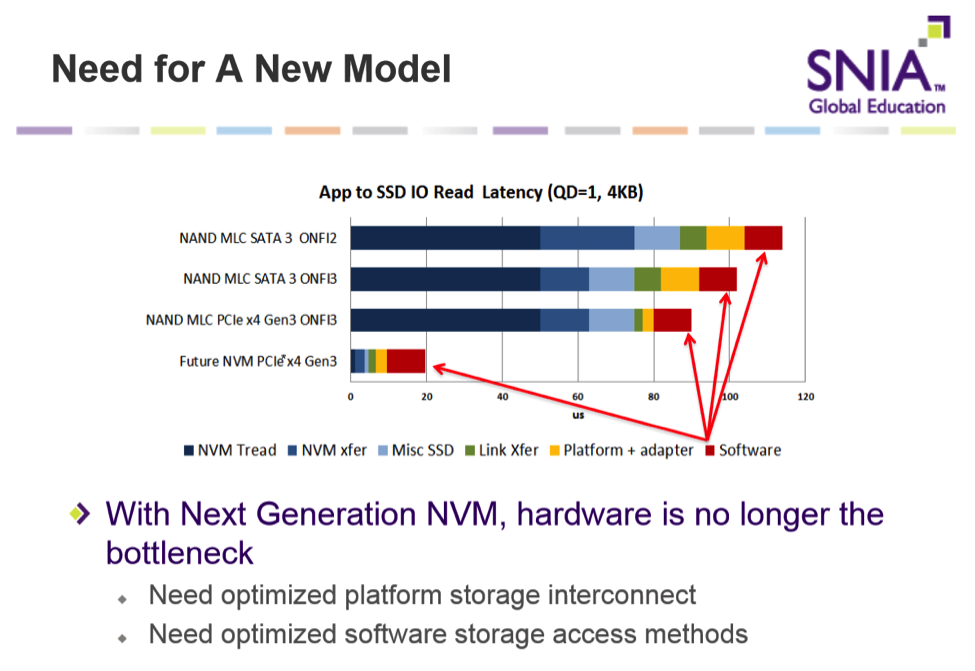
Q: Did All flash arrays almost eliminate bottleneck..,at least the Storage controller bottleneck can be eliminated if enterprise can afford all flash arrays?

A: Ken: Actually, almost exactly the opposite. Spinning drives are (now, at least) relatively slow. Over the past 10 years the drives have gotten much bigger, although HDD drive speeds haven’t really changed all that much,. Because of this, what I’ve observed is that the IOPS/GB ratio for HDD has, if anything, been getting worse* and the most common bottleneck for an HDD-based customer turns out to be the speed of their drives.

Now consider what happens when a customer moves to SSDs. The SSDs that are sold (and folks can afford) are generally much smaller than the HDDs they are used to, so customers buy as many of them as they can in order to meet their capacity requirements. And the SSDs are, one-for-one, much faster. So what happens? High drive counts + really fast drives = the drives aren’t your bottleneck anymore. Instead, the bottleneck shifts upstream … in a well architected solution, generally to the storage controller or clients.

*For those that know the terms, we could have a long discussion about working set sizes over the years, how fast data ages, tiered storage and such, and the effect that these have on observed iops/GB … but I think we could agree that since HDD speeds aren’t increasing, the iops/GB ratio isn’t generally getting better.

Q: Can I download this slides?

A: Ken: Absolutely. Here are the links to Part 1 of our series:

PPT and PDF: http://www.snia.org/forums/esf/knowledge/webcasts (look for “Storage Performance Benchmarking: Introduction and Fundamentals (July 2015)”)

Presentation Recording: https://www.brighttalk.com/webcast/663/164323

Q&A Blog: https://sniansfblog.org/?p=447

Here are the links to Part 2:

PPT and PDF: http://www.snia.org/forums/esf/knowledge/webcasts (look for “Storage Performance Benchmarking: Part 2 (October 2015)”)

Presentation Recording: https://www.brighttalk.com/webcast/663/164335

Q&A Blog: That’s what you’re reading now. 🙂

Q: Storage controller, is a compute node, right? And for hyper converged systems, storage controller and compute nodes are the same, right?

A: Mark: Most certainly, a Storage Controller can be a compute node, but in our webcast it is not. The term “compute node” is typically interpreted to be a part of the client/hosts layer. A compute node computes for the application, and such application is generating the workload (please see the question above about where workload is initiated).

A good example of the compute node would be a system that renders cartoons, or geodesic fields. As such compute node computes something (application does the work), and stores the results onto the storage controller.

However, in the case of hyper-converged infrastructure, the storage controller is often virtualized among the client hosts, making every compute node a part of a larger storage controller.

Q: Are the performance numbers that vendors publish typically front-end?

A: Mark: I don’t want to generalize published numbers as being one way or another. I recommend reading every publication for specific details. Vendors publish numbers to cover use cases, and each use case may come with its own set of expected measurement points and metrics. Ken and I talked about how metrics matter in the first Storage Performance Benchmarking webcast. 🙂

Q: “We did an R&D PoC using 32 flash 400GB elements attached on DIMM slots (not through SAS controller, not a direct PCIe attach) and seven 40Gbps cards. We were able to pump 5.5M 4KB-IOPS resulting in 30GB/s (240Gbps) of traffic on the front-end connect. When do you expect the front-end connect be the bottleneck for more standard environment?”

A: Ken: Woot! That sounds like a lot of fun. If you’re in the Raleigh, NC area and can talk about that not under NDA, we should have lunch. I’d like to hear more.

I have a suspicion that this answer won’t satisfy you, because it isn’t going to be as empirical as your example. The problem in answering with raw numbers is that there isn’t a standard configuration for a SUT. An enterprise class storage array with a mix of 40GbE and 32GB FC connections (with traffic over both) will look very different than someone using their old Windows XP box with a single 100Mbit to share out an SMB share, and both will look different than someone accessing their photos on their favorite cloud provider. So, I’ll answer the question by saying that I expect the front-end connect to be the bottleneck anytime the rest of the components in the SUT are capable of hitting your performance metrics (whether that be in terms of response time, IOPS, or data rates), and the front-end connect isn’t.

THAT said, you’d be astounded how often, even today, that MTU mismatches result in terrible front-end performance (and functionality).

Q: “Example of cache in front end connection?”

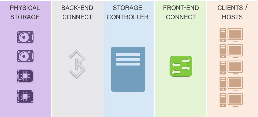
A: Ken: I’ll cheat and note that SUTs can be a lot more complicated than we showed. For example, our picture looked like this:


Benchmarking Image 1

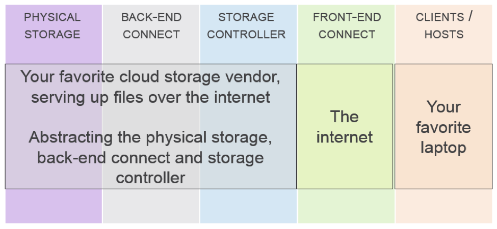
Consider a SUT then where you have:

Benchmarking Image 2

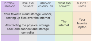
At one level, “the internet” is just a big black box acting as our front-end connect. But if we zoom in on it, perhaps we find that somewhere along the line there’s a caching server. Then we have an easy answer to where you find cache in the front-end connect.

In the much simpler model that you’ll find in many enterprise data environments though, you’ll find that the front-end connect consists of some relatively short length cables and a set of switches – either SAN or NAS switches. And in those environments, you won’t find a lot of cache. You will find memory, but you’ll find it used for buffering more than for caching.

We tried to minimize this in the presentation since there’s not a universally agreed upon distinction between these two terms. I think of a buffer (in this context) primarily as memory set aside to hold data very briefly, after which it is consumed and removed from the buffer. I think of cache, on the other hand, as a storage medium that holds data specifically to speed up data access (storage or retrieval). Data held in a cache can be held for a very long time, and not all data in a cache may ever be consumed/used.

Q: Even SSDs suck at random write but they are good for random read, is there that much difference?

A: Ken: Yes. The data we pulled for drive speeds was real data. And keep in mind that “sucks” is pretty relative here. Enterprise SSDs still tend to be at least 4x faster than spinning media. And, very importantly, their performance is much more consistent and deterministic since seek time is irrelevant with an SSD. New NVRAM technologies, like 3D XPoint, promise to dramatically improve write performance.

DRAM is volatile though so replacing HDDs with that wouldn’t really work, right? But if capacity requirements are high, we cannot replace disks with the cache, right?

A: Mark: Cache should never replace capacity. Cache is temporary storage, and requires by design to move its data to a permanent storage location. The size of cache should be matched to the size of the data that application uses, so called “working area”. For example, if an application writes to a 4GB file (think VMware vmdk), then for best performance the entire 4GB should fit into cache. However, capacity requirements for a VMware datastore can be as high as several TB. If the application (ESX server) is running many VMs, perhaps only the performance few need to fit into cache, while all other VMs would use cache for sub-portions of their vmdks.

A: Ken: You’re right, not permanently. As Mark points out, it isn’t to permanently replace the slower storage with cache necessarily, just supplement it enough that the working set fits in.

Q: How can we make client do less IO? Will it make sense?

A: Mark: A client does less IO by using larger IO size, for example. A classic use case is read- and write-sizes within NFS protocol. It is possible to increase read- and write-size of the NFS protocol from the NFS client mount options side. By default, some Linux environments use 32KB for reads and writes. And reading a 1GB file takes 32768 32KB IOs. If the read size is increased to 1GB, then it takes only 1024 IOs – a 32x reduction!

A: Ken: Other options involve app re-writes (yes, sometimes these ARE possible) and OS upgrades. Perhaps in the “app-rewrite” category, or maybe a new category, I’ve also worked with developers to rewrite their DB queries to be much less disk intensive, for example.

Q: Can you elaborate on some of the client level cache types other than file system or OS?

A: Mark: Other than file system and OS? Hmm… Let’s see: PCI-based cards that cache block-device level cache, e.g. EMC VFCache, SanDisk Fusion-IO, NetApp Flash Cache. Native network protocols (CIFS and NFS) caches. Local database caching, e.g., SafePeak, TimesTen, Windows Azure Caching.

Q: Please add more sessions, which goes into every detail

A: Mark: Absolutely! We will! Promise! We’re shooting for Part 3 in Q1 2016.

Update: This webcast is part of a series on storage performance benchmarking. Check out the others:

Life of a Storage Packet (Walk): Q&A

We got a lot of great questions at our recent Ethernet Storage Forum webcast “The Life of a Storage Packet (Walk).” As promised, we’ve compiled all the questions with fairly detailed answers. We hope this blog helps to clear up any confusion or uncertainties. If you think of additional questions, please comment below and we’ll get back to you as soon as we can. Thanks to everyone who watched the live webcast. If you missed it, it’s now available on-demand.

Q. Does size of a block depend on OS?

A. Yes, some OS’ only support 512 byte blocks. Some OS’ provide a method to support both 512 byte blocks and 4096 (aka 4K) byte blocks; for example, via a qualifier in their format command. Some devices are built using 4K block sizes, but then emulate 512 byte blocks to the host (aka 512E devices). Many modern versions of OS’ automatically detect the block size of each device they discover and do the right thing based on what they discover. You have to check the documentation for your OS to know its capabilities.

Q. CIFS is not a file system.

A. Not in the same way that ext, ntfs, FAT, HFS, UFS, etc. are, no. However, in terms of certain functionalities that we discussed on the presentation – that is, the ability to manipulate files with operations such as read, write, create, delete, and rename – are all file system functionalities. The difference being, of course, that the files are not on the local computer and are actually on a remote computer.

For what it’s worth, the term ‘CIFS’ has been deprecated from usage, and SMB is the preferred term for precisely the reasons that it should not be confused with local OS systems like the ones mentioned above.

Q. Is it safe to say that a “block” at the file system level is equal to an IO?

A. Not specifically. The difference in the use of those terms, is that a “block” is a place that data is stored – it has an address and it contains data (512 byte of data or 4K bytes of data). An IO is an operation that requests access to a block. An IO may perform a read operation on a block, or it may perform a write operation on a block.

Remember, the term IOPS is I/O operations per second – so it is not about blocks or bytes or bits – it is operations. If the operations are performed on a 512 byte block, they produce a different number of MB/sec than if they operate on a 4K byte block.

So, let’s take an example. A 1MB/second bandwidth on a 4K block size device is the same speed as 1MB/second bandwidth on a 512 byte block size device (observe, however, that the 4K block size device will have only 1/8 the IOPS that the 512 byte device has – because it will take only 1/8 the operations to transfer the same number of Mega-bytes). However, 1M IOPS on a 4K block size device is much better than 1M IOPS on a 512 byte block size device (because the 4K block size device is moving 8X the amount of data than the 512 byte block size device in each operation.

There is an excellent explanation and walk-through of IOPS in our Storage Performance Benchmarking webinar.

Q. Don’t all those Inodes also live on the disk and so don’t the IOs to read those blocks also have to go to the SCSI controller?

A. Well-spotted!

The communication back and forth between the file system and the Inodes traverses the controller for all access to blocks on disk. This is one of the reasons why needing to access disk is considered “expensive.” When you add in a network to the mix, these kinds of situations need particular careful consideration.

Q. Shall we allocate blocks and inodes or is it an automatic process?

A. It’s an automated process, and there is no user intervention at all.

Q. Are Inodes created during OS installation?

A. Inodes are a particular block type, among some other block types (e.g., data blocks, boot blocks, superblocks, group descriptor blocks). These block types are combined into functional groups. These groups are OS-dependent. The block layout therefore, including Inodes, is created during OS installation. If the filesystem needs more Inodes after the OS installation, the OS dynamically adds them to the Inode pool.

Q. Which physical hardware does volume manager reside?

A. Volume managers are not hardware. They are software layers that create pseudo devices that are presented to layers of the OS above them (typically to the file system layer). The volume manager software fits into the OS to accept requests from the file system and pass those requests down to the device driver. In some systems they might be called “filter drivers”.

Q. In flash media, is there also an iSCSI controller that converts PCIe into iSCSI to interact with the flash?

A. I want to make sure that the answer to the question is clear.

On the host, we need to convert PCIe commands to SCSI, so we send them to an iSCSI controller/adapter to be sent across the Ethernet wire. . That adapter can be either software or hardware.

Flash drives are basic media, just like spinning disk drives. Flash will have its own controller, which can be SCSI. If you wish to access the drive over Ethernet using the iSCSI protocol, you will have an adapter on the flash drive (which can be either software or hardware) that will do the SCSI translation between the Flash media and the SCSI commands. This is often called the FTL – or the flash translation layer. Again, the SCSI commands are translated into an Ethernet-friendly packet to be sent along the wire.

There are other types of communication forms for working with Flash, too. The most recent is NVMe. You can see the SNIA webinar on The Performance Impact of NVMe and NVMe over Fabrics for more information.

Q. Why is there a SCSI language in between Storage and the hosts?

A. Before storage standards (like SCSI and ATA), you would purchase storage from Vendor X, and you would also buy a storage controller for that vendor X storage.   If you wanted Vendor Y storage, you could not use the vendor X controller, you had to purchase a new controller from vendor Y. Every vendor had their own language, and you had to purchase matching components.   Once you got locked into one vendor, you were stuck – at the hardware level.

Today with standards (such as SCSI), you can buy a SCSI device from any vendor and connect it to any storage controller that you buy from any vendor – and it just works.   That is the point of the SCSI standard. When the storage standardization efforts began, there were many competing ideas. It just so happened that SCSI won out, and so now it’s everywhere.

Q. If the storage side is flash, do we still need a SCSI controller between host and flash storage or is the controller different for a flash storage?

Yes… and no.

Yes, to use the SCSI part of the OS, the flash device must continue to speak the SCSI protocol and so a SCSI controller is needed. This method of communicating with flash devices enables all the existing S/W on the host OS to just continue working without even knowing it is flash.

No, flash memory chips can be connected to the system using non-SCSI methods. Most of those methods are generally special purpose applications and so the existing OS S/W simply cannot use that device (only the special purpose S/W designed for that device can use it). However, NVMe is a new protocol that is enabling more general use of the flash memory technology with the hopes to provide new capabilities that are beyond what SCSI provides. This is also discussed in our webcast on The Performance Impact of NVMe and NVMe over Fabrics.

Q. What’s the difference between partition, logical disk, volume, LUN, etc?

Excellent question!

Let’s work this one backwards – LUN – that is a SCSI term (actually an acronym) that refers to the Logical Unit Number – it is part of the address used to access a logical unit. Small SCSI devices (such as a single spindle disk drive) have only a single logical unit. Large storage arrays may contain 100s of logical units. Each of those logical units appears to the host OS as if it were a single spindle disk. So, the logical unit is the SCSI object that contains the blocks where the data is stored (where that object may be an individual piece of hardware, or a logical entity within a larger SCSI device). To access a SCSI logical unit, the OS must specify the address of the SCSI device, and then the LUN (logical unit number) for the logical unit within that SCSI device.

The other terms (partition, logical disk, and volume) are OS terms that have to do with virtualization and how the storage blocks are managed. When a SCSI (or other storage device) is formatted by the OS, it may be broken into multiple partitions. Each partition is then treated by the OS as if it were a unique device (a virtual device, or a logical disk). Each of those partitions may then be used independently.

For example, on a Unix system, the “a” partition may contain a file system that has all the files that are necessary to boot. The “b” partition may be setup without a file system and used as the swap or paging storage for use by the virtual memory subsystem. The “d” partition may then contain a file system that contains all the user’s data files. Each partition is unique storage space and may even use a different file system to organize the data located there.

Notice, that I skipped the “c” partition. That partition is often setup to access all the blocks of the physical device. So, on a 500GB disk, maybe “a” contains 10GB, “b” contains 90GB, and “d” contains 400GB; while “c” contains all 500GB. Partitions “a” and “d” may be backed up or restored independently, and partition “c” may be used to perform an image copy of the entire device.

Now, to the other terms:

Logical disk and volume are terms often related to volume managers.

  • Logical disk may be a term used to refer to a partition, but usually that is not the case. Logical disks are typically the devices created by the volume management layer when they combine individual devices into a single larger device (a.k.a. a logical disk).
  • Volume managers also may be used to divide up a large device into small chunks (just like partitions), and those smaller chunks are referred to as logical disks.
  • Volume is a more vague term that typically is used as another term for a logical disk. In some circles, the term Volume is used to refer to a RAID set in a SCSI storage controller (but this is a much less often used definition for Volume).

Q. Will the “complete” presentation somewhere we can go review?

Yes. Click here to access the on-demand webcast as well as a PDF of the webcast slides

Update: If you missed the live event, it’s now available  on-demand. You can also  download the webcast slides.

New Webcast: The Life of a Storage Packet (Walk)

Wonder how storage really works? When we talk about “Storage” in the context of data centers, it can mean different things to different people. Someone who is developing applications will have a very different perspective than someone who is responsible for managing that data on some form of media. Moreover, someone who is responsible for transporting data from one place to another has their own view that is related to, and yet different from, the previous two.

Add in virtualization and layers of abstraction, from file systems to storage protocols, and things can get very confusing very quickly. Pretty soon people don’t even know the right questions to ask! That’s why we’re hosting our next SNIA Ethernet Storage Webcast, “Life of a Storage Packet (Walk).”

Join us on November 19th to learn how applications and workloads get information. Find out what happens when you need more of it, or faster access to it, or move it far away. This Webcast will take a step back and look at “storage” with a “big picture” perspective, looking at the whole piece and attempting to fill in some of the blanks for you. We’ll be talking about:

  • Applications and RAM
  • Servers and Disks
  • Networks and Storage Types
  • Storage and Distances
  • Tools of the Trade/Offs

The goal of the Webcast is not to make specific recommendations, but equip you with information that will help you ask the relevant questions, as well as get a keener insight to the consequences of storage choices.  As always, this event is live, so please bring your questions, we’ll answer as many as we can on the spot. I encourage you to register today. Hope to see you on November 19th!

Update: If you missed the live event, it’s now available  on-demand. You can also  download the webcast slides.

Storage Performance Benchmarking Q&A

Our recent SNIA-ESF webcast, “Storage Performance Benchmarking: Introduction and Fundamentals” really struck a chord! It was our most highly rated and well attended webcast to date with more than 300 people at the live event. If you missed it, it’s now available on-demand. Thanks again to my colleagues, Ken Cantrell and Mark Rogov, who did an outstanding job explaining the basics and setting the stage for our next webcast in this series, “Storage Performance Benchmarking: Part 2” on October 21st. Mark your calendar! Our audience had many great questions and there just wasn’t enough time to answer them all, so as promised, here are answers to all the questions we received.

Q. Can you explain the difference between MiB and MB?

A. The difference lies between the way that bytes are calculated. A megabyte (MB) is defined in decimal (base-10), and a mebibyte (MiB) in binary (base-2). There is a similar relationship between kilobytes (base-10) and kibibytes (KiB). So, if you begin with a single byte:

1 kilobyte (KB) = 1000 bytes (B)

1 kibibyte (KiB) = 1024 bytes (B)

1 megabyte (MB) = 1000 KB = 1000 * 1000 bytes = 1,000,000 bytes

1 mebibyte (MiB) = 1024 KiB = 1024 * 1024 bytes = 1,048,576 bytes

The distinction is important because very few applications or vendors make use of the MiB notation and instead use the MB notation to refer to binary numbers. If vendor or tool A is using MB to refer to base-10 measurements, and vendor or tool B is using MB to refer to base-2 measurements, it may falsely appear that the two vendors or tools are performing differently (or the same), when in fact the difference (or similarity) is simply because they are labeling two different things (MB and MiB) as the same (MB).

Telecommunications and networking generally measure and report in MB.  Disk drive manufacturers tend label storage in terms of MB. Many operating systems report storage labeled as MB, but calculated as MiB.  Storage performance (whether from an application’s view, or the storage vendor’s own tools) is generally measured in binary (MiB/s), but reported in decimal (MB/s).

Q. I disagree with the conflation of the terms “IOPS” and “throughput.” Throughput generally refers to overall concept of aggregate performance. IOPS measure throughput at a given request size, which most clients assume to be small blocks (~512B-4K). Many clients would say that bandwidth, measured in MB/s or GB/s, is a measure of throughput @ large block size (>~128K). Performance typically varies significantly @ different block sizes. So clients need to understand that all 3 of these concepts differ.

A. The SNIA dictionary equates throughput to IOPS, which is why we listed it as a common alternative for IOPS.   However, the problem with “throughput” is in the industry’s lack of agreement on what this term means. See the examples below, where sometimes it clearly refers to IOPS and other times to MB/s.   This is why, in the end, we recommend you simply don’t use the term at all, and use either IOPS or MB/s.

Throughput = MB/s

Techterms.com:  “Throughput refers to how much data can be transferred from one location to another in a given amount of time. It is used to measure the performance of hard drives and RAM, as well as Internet and network connections.”

Meriam-Webster:  “The amount of material, data, etc., that enters and goes through something (such as a machine or system)”

Throughput = IOPS

SNIA Dictionary: “Throughput:   [Computer System] the number of I/O requests satisfied per unit time.     Expressed in I/O requests/second, where a request is an application request to a storage subsystem to perform a read or write operation.”

Wikipedia:   “When used in the context of communication networks, such as Ethernet or packet radio, throughput or network throughput is the rate of successful message delivery over a communication channel. The data these messages belong to may be delivered over a physical or logical link, or it can pass through a certain network node. Throughput is usually measured in bits per second (bit/s or bps), and sometimes in data packets per second (p/s or pps) or data packets per time slot.”

TechTarget:   “Throughput is a term used in information technology that indicates how many units of information can be processed in a set amount of time.”

Throughput = Either

Dictionary.com:   “1. The rate at which a processor can work expressed in instructions per second or jobs per hour or some other unit of performance. 2.  Data transfer rate.”

Q. So, did I hear it right? IOPS and Throughput are the same and thus can be used interchangeably?

A. Please see definitions above.

Q. The difference between FE/BE is the raid level + Write percentage = overhead IOPS. It is different at times due to RAID or any virtualization at the storage level, like if you have RAID 5, every front-end write would have 4 backend write. What happens if the throughput at the back end of a controller is more than at the front end?

A. The difference between Front End (FE) and Back End (BE) is generally the vantage point. One of the objectives of the presentation was to show that when comparing two results (or systems) the IOPS must be measured at the same point. BE IOPS depend, in part, on the protection overhead and on the software engine’s ability to counteract it. But instead of defining why there is a difference, we aimed at exposing that such difference exists. The “whys” will be addressed in the future webcasts.

Q. Also, another point that would dictate which system is the storage capacity each has to offer. Very good compare & contrast illustration.

A. Agreed, although capacity itself has several facets: raw capacity or the sum of manufacture advertised capacities of all internal drives; usable capacity or the amount of data that could be written on one system after all formatting and partitioning; and logical capacity or the amount of data that external hosts could write onto the system. Logical may be different from usable based on some data reduction services that a system could offer.

Q. Why is there a lower limit on your acceptable latency band? Storage can be too fast for your business needs?

A. We had some discussions looking at whether you show it as a cap, or a band. In many cases, customers will have a target latency cap, but allow some level of exceptions (either % of time it is exceeded, or % by which it is exceeded). That initially suggested a soft cap and a hard cap. One of us also has seen customers that highly value consistent behavior. In a service provider context, providing “too fast” performance could actually build a downstream customer expectation that will cause satisfaction issues if performance later degrades, even if it degrades to levels within the original targets.   You could certainly see this more generally as a cap though, which Ken stated verbally in the presentation. The band represents not only the cap, but also variance.

Q. What is an “OP”? An”Operation Per”? Shouldn’t this be “$/OPS” or “dollars per operation per second”?

A. This question was raised during the verbal Q&A. An “OP” in our context was any of the potential protocol-level operations. For example, in an NFSv3 context, this could be a CREATE, SETATTR, GETATTR, or FINDFILE operation. The number of these that occur in a second is what we referred to as OPS. There is certainly potential confusion here, and we struggled for consistency as we put the presentation together.

For example, sometimes we (and others) refer to operations per second as “op/s” instead of OPS, or use “Ops” or “OPs” or “ops” to mean “more than one operation” instead of “operations per second.” We chose to use OPS because it is consistent with IOPS, which we see frequently in this space, and are trying to push others towards this terminology for consistency.

Q. More IOPS in the same amount of time seems to imply that the system with more IOPS is performing each IO in less time than the other system. So how do we explain a system that can do more IOPS than another system but with a higher response time for each IO than the other system?

A. Excellent question! Two different angles on a reply follow …

First angle:

A simple IOP count doesn’t include the size of the IOP, or the work that the storage controller must perform to process it. Therefore comparing just the IOPS does not provide a good comparison: what if system 1 was doing large IOs (64KiB or more) and system 2 was doing small IOs (4KiB or less)? To avoid that, most people fix the IO size or run controlled tests changing the IO size in steps and then compare the arrays.

The point that we are making with the webcast is that IOPS alone are not enough for a comparison, one must look beyond that into IO size, response time and above all business requirements.

Second angle:

This is an excellent question, and there are at least two answers.

To begin, we need to explain the relationship between IOPS and response time.

We generally talk about response time (latency) in terms of seconds or milliseconds. We say things like “a response time of 5ms.” But this is actually a shortcut. It is really “seconds per I/O” or “milliseconds per I/O.” Also, remember that in “IOPS” the “p” stands for “per”, so this is “IOs per second.” So, ignoring the conversions between “seconds” and “milliseconds”, the relationship between IOPS and response time is easy…they are inverses of each other:

blog image 1

So:

blog image 2

Implies:

blog image 3

Example:

blog image 4


blog image 5

Given this:

The first answer to your question is tied to idle time. Consider the following simple example.

System 1:

For system1, assume that the storage array service time is the only significant contributor to latency.

Client issues an I/O

Storage array services the I/O in 10ms

As soon as the client sees the response, it immediately issues a new I/O

Process continues, with all I/Os serviced by the storage array in 10ms each

How many IOPS is system 1 doing?   Measured at the client, or the storage array, it is doing 100 IOPS with an average response time of 10ms.   Remember the relationship between IOPS and response time from the intro above.

System 2:

For system2, assume that both the client and storage array contribute to latency.

Client issues an I/O

Storage array services the I/O in 5ms.

Client waits 5ms before issuing a new I/O.

Process continues, with all I/Os being serviced by the storage array in 5ms each, and the client waiting 5ms between issuing each I/O.

How many IOPS is system2 doing? If you measure the total number of I/Os completed in a minute, it is completing the same # as System1 and so doing 100 IOPS. But what is the latency? If you measured the latency at the storage array, it would be 5ms. If you measured at the client, it would depend on whether your measurement was above or below the point where the 5ms delay per I/O was inserted, and would see either 5ms or 10ms.

The second answer is tied to “concurrency,” an element we didn’t discuss in the webcast.

Concurrency might also be called “parallelism.”  In the examples above, the concurrency was ‘1′. There was only ‘1′ I/O active at a time.

What if we had more though?   Example:

For both systems, assume that the storage array service time is the only significant contributor to latency.

System 1 (same as above)

Client issues an I/O

Storage array services the I/O in 10ms

As soon as the client sees the response, it immediately issues a new I/O

Process continues, with all I/Os serviced by the storage array in 10ms each

How many IOPS is system 1 doing?   Measured at the client, or the storage array, it is doing 100 IOPS with an average response time of 10ms. Remember the relationship between IOPS and response time from the intro above.

System 2:   Increased concurrency

Client issues two I/Os

Storage array receives both and is able to handle both in parallel, but they take 20ms to complete

As soon as the client sees the response, it immediately issues two new I/Os

Process continues, with all I/Os serviced by the storage array in 20ms each, and the client always issuing two at a time

How many IOPS is system 2 doing? In the aggregate, measured at the client or the storage array, it is doing 100 IOPS. What is the response time? This is where the relationship between IOPS and response time introduced before can break down, depending on what you’re really asking for and it really takes some queuing theory to properly explain this. Ignoring the different kinds of queuing models and simplifying for this discussion, at a high level you could say that the average response time is still 10ms. Some reporting tools are likely to do this. That is misleading however, since each I/O really took 20ms. You’d only see a 20ms response if (a) you actually kept track of the real response times somewhere [which many systems do … they’ll create many different response time buckets and store counts of the # of I/Os with a given response time in a given bucket], or (b) you make use of Little’s Law. Little’s Law would at least give you a better mean response time. We didn’t discuss Little’s Law in the webcast, and I won’t go into much detail of it here (follow the Wikipedia link if you want to know more), but in short, Little’s Law can be rearranged to state that:

blog image 6

or, in our case above:

blog image 7

Q. What is valuable from SPEC’s SFS benchmark in this context?

A. Excellent question. We think very highly of SPEC SFS © 2014 for a variety of reasons, but in this context, a few stick out in particular:

1) The workloads provided by SPEC SFS 2014 are the result of multi-vendor research, actual workload traces, and efforts to target real business use cases. The VDI (virtual desktop infrastructure), SWBUILD (software build), DB (OLTP database) and VDA (video data acquisition) workloads are all distinct workloads with very different I/O patterns, I/O size mixes, and operation mixes. We’ll talk more in another session about these aspects of a workload, but the important element is that each workload is designed to help users understand performance in a specific business context.

2) To encourage folks to think in a business context, SPEC SFS 2014 primarily reports results  not  in IOPS or MB/S, but in the relevant “business units” at a given response time, along with a measure of overall response time, aptly referred to as ORT (Overall Response Time).   For example, the SWBUILD workload reports load points as “number of concurrent software builds.” MB/s information is still available for those that want to dig in, but what is really important is not the MB/s, but how many software builds, or databases, or virtual desktops, or video streams can a system support, and this is where the reporting focus is.

3) SPEC SFS 2014 recognizes that  consistent  performance is generally an important element of  good performance. SPEC SFS 2014 implements a variety of checks during execution to make sure that each element doing I/O is doing roughly the same amount of I/O and that they are doing the amount of work that was requested of them and aren’t lagging behind.

More information on SPEC SFS 2014 (and SPEC in general) is available from  http://www.spec.org

Q. Anything different/special about measuring and testing object storage?

A. Object Storage is a hot topic in the industry right now, but unfortunately fell outside the scope of this fundamentals presentation. We will be examining object storage – and corresponding network protocols – in a later webcast. Stay tuned!

Q. Does Queue depth not matter in response times?

A. We did not define Queue Depth as a term in this webcast because we classified it as an advanced subject. We are planning to address queue depth during a future webcast. In short, the queue depth does play an important role in the performance world, but response time is affected by it only indirectly. When the target Queue is full, the Initiator can’t send any more IOs and waits for the Queue to free up.

The time spent waiting is not response time. Response time measures the time the Target spends processing the IO it was able to receive (place into its queue). However, some scenarios may keep an IO inside a Queue for a long time (due to storage controller doing something else), and thus increase the response time for the waiting IO. In the latter case, increasing the depth of the Queue will increase the response time.

Keep in mind thought that “It Depends”. It depends on where you measure. For example, a client may have no visibility into what is happening at the storage array. It cares about how long the storage array takes to respond … it doesn’t know or care about the differences between the storage array’s view of its service time (how long the storage array is doing work) and its queuing delay / wait time (how long it is waiting to do work).

As far as the client is concerned, this is all response time. It just wants a response. Most “response time” metrics reported by tools / apps/ storage arrays really decompose into a set of true service times and queuing delays, although you may never get to see how those components come together w/o using other tools.

Q. Order is important, in addition to mix ratios. For IOs, sequential vs. random (and specifics on randomness) is important. For file operations, where the protocol is stateful, the sequence of operations can strongly impact performance. Both block and file storage can have caches, which behave very differently depending on ordering and working set size. I suggest including the concept of order in a storage benchmarking intro.

A. These are excellent points, but given the amount of time we had, we had to make some hard choices about what to include and what to drop (or defer). This fell on the chopping block. Someone once told me that the best talks are those where you cry over what you’ve been forced to leave on the cutting room floor. There was a lot of good stuff we couldn’t include. I expect that we will address this idea in the planned discussion of workloads.

Q. The “S” in “OPS” and “IOPS” means Seconds and isn’t a pluralization. Some people make a mistake here and use the term “OP” and “IOP” to mean “1 operation/second” or “1 IO/second”. This mistake happens in this presentation, where “$/OP” is used. The numbers suggest what was intended is “# of dollars to get 1 operations/second.” The term “$/OP” can be misinterpreted to mean “dollars per operation,” which is a different but also relevant metric for perishable storage, like flash.

A. Good catch. We tried hard to be consistent in using “OPS” instead of “op/s” or some variant, when we meant “operations per second”.  There is another Q&A that addresses this. Technically, we slipped up in saying “$/OP” instead of “$/OPS” when we meant, as you noted, “Dollars per (operations per second)”. That said, I think you’ll find that nearly everyone makes this shortcut/mistake. That doesn’t make it right, but does mean you should watch out for it.

Q. Isn’t capacity reported in MiB, Gib etc and bandwidth in MB/s today?

A. Unfortunately, our impression is that capacity is also reported in decimal, at least in marketing literature. All we were trying to point out is that units of measurements must be consistent at all points. Many people mix decimal and binary numbers creating ambiguities and errors (remember that at a TiB vs. TB level, the difference is 10%!) For example, graphs that show IO size in decimal and bandwidth in binary.

Q. Would you also please talk about different SAN protocols and how they differ/impact the performance?

A. There are additional webcasts under development that discuss the storage networking protocols, their performance trade/offs, and how performance can be affected by their use. Due to time constraints we needed to postpone this portion because it deserves more attention than we could provide in this session.

Q. So even though IOPS could be more, the response time could be less…so it’s important to consider both. Is that correct?

A. Absolutely! But just response time is not enough either! You need more load points, and a business objective to truly assess the value of a solution.

Update: This webcast is part of a series on storage performance benchmarking. Check out the others:


New Webcast: Storage Performance Benchmarking 101

There’s an art to making sense of storage performance benchmarks. That’s why ESF is hosting a live Webcast on this important topic. Please join us on July 30th for “Storage Performance Benchmarking: Introduction and Fundamentals.”     At this Webcast, you’ll gain an understanding of the complexities of benchmarking modern storage arrays and learn the terminology foundations necessary for the rest of the series as Mark Rogov, Advisory Systems Engineer at EMC, Ken Cantrell, Performance Engineering Manager at NetApp, and I discuss:

  • The different kinds of performance benchmarking engagements
  • An introduction to the variety of relevant metrics
  • How to determine the “right” metrics for your business
  • Terminology basics:  IOPS, op/s, throughput, bandwidth, latency/response time

If you’re untrained in the storage performance arts, this Webcast will bring you up-to-speed on the basics. My colleagues and I hope it will be an informative and interactive hour. Please register today and bring your questions. I hope to see you there.

Update: This webcast is part of a series on storage performance benchmarking. Check out the others:

The Life of a Storage Packet

Keeping storage as close to the application as possible and reasonable is important, but different types of storage can make a big difference for performance as well as types of workloads. Starting with the basics and working to more complexity, find out how storage really works in this first of the Packet Walk series of the “Napkin Dialogues” series. Warning: You’re on your own when tipping the pizza delivery person!

Download (PDF, 1.71MB)